
University of Piraeus
School of Information and Communication Technologies
Department of Informatics
Applications of NEAT algorithm for automatic gameplay of agents in deterministic and non-deterministic game environments
Acknowledgements
This project was a life experience for two reasons: first, due to the vast research and knowledge it offered and second, because it was concluded during the coronavirus pandemic. My senior year as a student ended abruptly right before finishing my undergraduate studies. Regardless, after hours of reading, discussing, brainstorming and programming, I am excited to have finished this project.
I would like to thank my professor Dr. Dionisios Sotiropoulos for accepting my original proposition for the subject and guiding me during this time. I would also like to thank my parents John and Maria, for motivating me to keep up the hard work and bearing with me during the quarantine. Lastly, I want to express my gratitude for SethBling, an American YouTuber for publishing the video "MarI/O – Machine Learning for Video Games"which was my original inspiration for the subject of this project.
Abstract
On this project, we study applications of the NEAT algorithm in deterministic and non-deterministic game environments. First, we look at an overview of the NEAT algorithm, how it works, design principles and the challenges that come with implementation. Next, we introduce a custom two-dimensional game in Python for two players: blue and red. We lay down the basic rules and structure, in order to create an environment suitable for neuroevolution. Finally, we study five training cases, where the blue and red player are given several tasks that must be achieved through the evolution of neural networks.
Contents
List of figures
- Figure 1.1 The phenotype (left) and genotype (right) of a neural network in NEAT
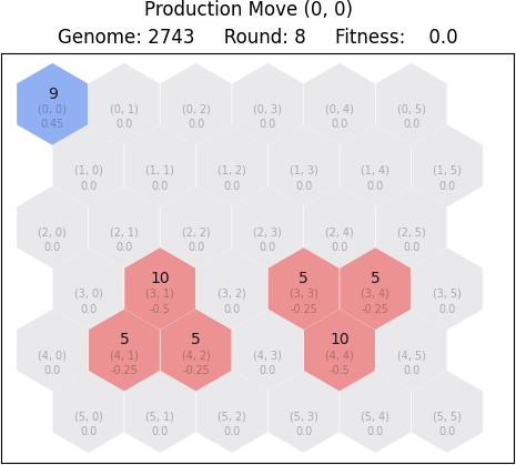
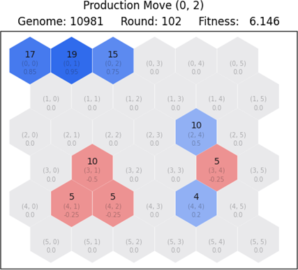
- Figure 2.1 Game state before a production move
- Figure 2.2 Game state after a production move
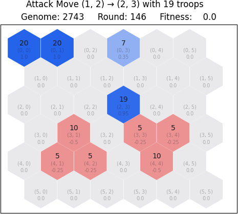
- Figure 2.3 Game state before an attack move
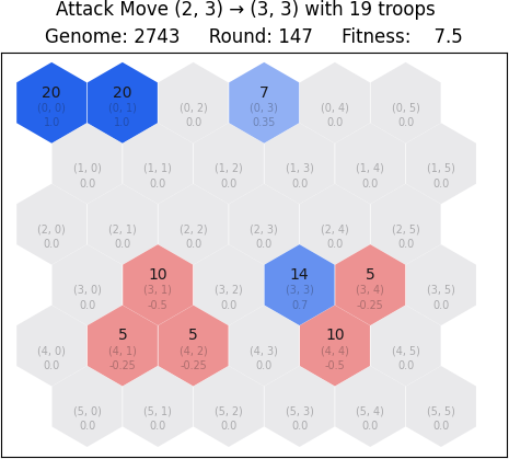
- Figure 2.4 Game state after an attack move
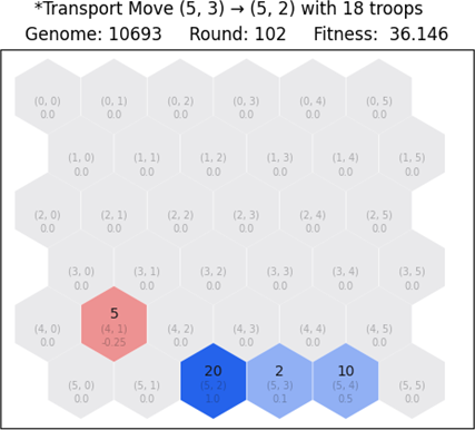
- Figure 2.5 Game state before a transport move
- Figure 2.6 Game state after a transport move
- Figure 3.1 An example game state representation with matplotlib
- Figure 5.1 Example game state of players starting from top left and bottom right
- Figure 5.2 Example game state after a considerable number of rounds
- Figure 5.3 The map_owners matrix representation from the Game class
- Figure 5.4 The map_troops matrix representation from the Game class
- Figure 6.1 The initial state of the first training case
- Figure 6.2 Fitness progression of the first training case
- Figure 6.3 End state of the most fit network for the first training case
- Figure 6.4 Example state of the second-best network for the first training case
- Figure 6.5 The initial state of the second training case
- Figure 6.6 Fitness progression of the second training case
- Figure 6.7 End state of the most fit network for the second training case
- Figure 6.8 Example state of the second-best network for the second training case
- Figure 6.9 Example state of the third-best network for the second training case
- Figure 6.10 The game state of the third training case
- Figure 6.11 Fitness progression of the third training case
- Figure 6.12 End state of the most fit network for the third training case
- Figure 6.13 Example state of the second-best network for the third training case
- Figure 6.14 Example state of the third-best network for the third training case
- Figure 6.15 Initial state for the fourth training case
- Figure 6.16 Fitness progression of the fourth training case
- Figure 6.17 The end state of the most fit network for the fourth training case
- Figure 6.18 The initial state for the fifth training case
- Figure 6.19 Fitness progression of the fifth training case
- Figure 6.20 Example intermediate state for the fifth training case
- Figure 6.21 Example end state for the fifth training case
1. Overview of NEAT algorithm
NeuroEvolution of Augmenting Topologies (NEAT) is an algorithm that is used to evolve neural networks through a novel method of genetic evolution [1]. Traditionally, the topologies of neural networks in neuroevolution (NE) use a fixed layout of neurons. The goal is to search through the weight space and find optimal values for a given problem. This task is achieved through a population-based stochastic search algorithm, where neural networks crossover to create ancestors with the intent of outperforming their predecessors. When mutations occur certain weight values are randomly modified. This allows for neural networks to gradually develop new behavior and better approximate the fitness function of a given problem [2].
The NEAT algorithm is different because both topologies and weights are evolved. The drive behind this novel method emerges from an importation question: can evolving topologies and weights provide a clear advantage over fixed topologies of evolving weights? If the behavior of neural networks depends on both topology and weights, it is evident that evolving both aspects is worth studying [3]. Starting off with an initial population, it is a design principle for topologies to be minimal. As generations progress, neural networks crossover and mutations occur on both structure and weights. This design difference is crucial because it allows for optimal solutions to be developed. Consequently, maintaining minimal topologies is proportional to minimizing search spaces, allowing for greater performance.
Of course, there are several challenges that come with this methodology. First off, topologies must be genetically represented in such a way that the competing conventions problem is addressed. When two structurally different neural networks present the same solution to a given task, it is likely that an offspring would be negatively affected [4]. Second, it is essential that structural innovations are preserved throughout the evolutionary process. Certain features sometimes require more than a few generations to develop, as neural networks gradually optimize their structure. Lastly, it is necessary for the whole process to come up with minimal solutions. For that to happen, neural networks must start out minimally and increase complexity if necessary. This can be achieved without the need of including a complexity component on the fitness function.
As with any NE algorithm, the weights of a neural network are subject to mutations. In NEAT, mutations also occur on connections and nodes. During this process, the algorithm assigns historical markings in the form of innovation numbers. That way, we can effectively keep track of all the different mutations and compare the genotypes of neural networks. To prevent exploitation of this system, cases of duplicate mutations are assigned the same innovation number. Genomes are composed of genes, a linear representation of connecting nodes. Genes are defined with an input node, an output node, the weight of the connection, whether it is active or disabled and the innovation number. A mutation that adds one node would insert two new genes of connectivity and disable the original one, whereas a mutation that adds a connection would simply insert a new gene for the two connecting nodes.
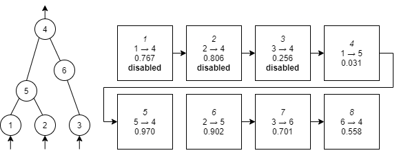
Keeping track of all the different mutations using innovation numbers, allows for great flexibility during the crossover stage. We know which genes came before, after or in parallel, therefore, the sequences can be compared. When two genomes are crossed over, we look at the genes that comprise their genotypes. There are three distinct cases during the alignment: matching genes, disjoint genes and excess genes. We assume that matching genes are inherited randomly, with a special case for disjoint and excess genes that come from the most fit parent. Enabled genes may become disabled, and disabled genes may be activated again. By initiating crossover after evaluating fitness, we end up with a diverse population of neural networks that express different types of features.
Applying structural mutations comes with a cost. By inserting new node and connection genes on the genotype of neural networks, their fitness might initially decrease. Because small networks tend to perform better, it is crucial that the algorithm takes extra care of complex structures. Large networks usually require more generations to optimize and yield a better fitness payoff. Having that in mind, we give large structures a fair chance by speciating the population.
Performing speciation on a diverse population is no easy task. The goal is to sort similar topologies under the same types of species. That way, instead of competing with the entire population, neural networks compete within their own niche. Thankfully, this process is simplified, because of how the genotypes are encoded. It turns out that similarities and differences found in the genotype is a natural way of measuring the compatibility of genomes. During each generation, genomes are assigned to a species based on a compatibility distance metric. The number of disjoint and excess genes along with the weight differences of matching genes is considered. Lastly, genomes within their own species reproduce based on explicit fitness sharing. The most fit genomes within the niche reproduce and the lowest performing genomes are discarded.
Before utilizing NEAT for this project, it is essential to look at benchmarks and check the validity of assumptions put forward. First, NEAT is tested against the problem of evolving a neural network capable of solving the XOR problem. Given that at least one hidden layer is required for a solution, it is fundamental that we can check whether NEAT can evolve such topologies. Next, NEAT is put to work on double pole balancing tasks. This benchmark is important because it resembles real life problems with adjustable difficulty. Several other NE systems use this scenario; therefore, the performance can be compared with ease. Finally, NEAT is tested against a series of ablations in order to verify the contribution to the overall performance of each individual component: historical markings, speciation and starting out minimally.
As it turns out, NEAT is more than capable of performing well on all benchmarks. For the XOR problem, the algorithm ran 100 times and converged to a solution after an average of 32 generations. The solution networks on average included 2.35 hidden nodes and 7.48 active connections. During all iterations, the algorithm was able to converge on all 100 runs, with the worst case of running for 90 generations. As for the double pole balancing challenge, the scenario is that the network must apply forces to a cart in order to keep the two poles balanced. There were two versions: double pole balancing with velocity (DPV) and double pole balancing without velocity (DPNV). On the DPV problem, NEAT was able to come first compared with four other NE systems: Evolutionary Programming, Conventional NE, SANE and ESP. On the DPNV problem, NEAT was once again, able to finish first compared with two other NE systems: CE and ESP. For both cases, the number of evaluations were less than all other methodologies.
After succeeding on all benchmarks, the NEAT algorithm was applied on the DPV problem with a series of ablations. First, NEAT is set to run without the ability of growing the structure of neural networks. Because all networks start minimally, for this ablation networks are initialized with 10 hidden nodes. After 20 runs, failure rate reached 80%. The second ablation forced networks to start with a random topology instead of initializing minimally. The number of hidden nodes is initially set between 1 and 10 with random connections. It turns out that NEAT was 7 times slower and failed to find a solution 5% of the time. The third ablation removed the feature of speciation. For this case, initial population is set to start out with random topologies to introduce needed diversity. It is observed that the algorithm failed 25% of the time and was 7 times slower. The last ablation removed mating of genomes. After 120 runs, it was concluded that the average evaluations were 5,557 compared to 3,600 if NEAT was applied normally.
In summary, NEAT is an efficient algorithm for artificially evolving neural networks. The main difference compared to other NE systems, is that both topology and weights are evolved, granting a significant performance boost. The XOR problem along with pole balancing tasks have demonstrated that NEAT can solve real world problems. Ablation studies have shown that the main key components of NEAT: historical markings, speciation and incremental growth all bond together to come up with minimal solutions. It is not only the end result that is important, rather, all intermediate solutions that contribute to the process. We conclude that NEAT reinforces the analogy between genetic algorithms and natural evolution, as it can optimize and complexify solutions at the same time.
2. Game Overview
Measuring the efficiency of neural networks in a turn-based strategy game, requires an environment where artificial players can declare moves and evaluate the outcome. For this purpose, a basic game framework was prototyped in Python. The framework allows for quick development of game presets with common rulesets that act as training grounds. Presets are used to create initial game states, where neural networks can unfold their strategy. Once the game is deemed to be over, the end state is evaluated, and the fitness is measured.
The game consists of two players, blue and red, where each one takes turns with the purpose of defeating one another. Each player is placed on a map of hexagons called tiles, that simulate different territories. Tiles have specific colors of ownership and a varying number of troops. Blue tiles are owned by the blue player and red tiles are owned by the red player. For convenience, gray tiles are assumed to belong in nature.
Tiles are considered owned when one or more troops are present. For a player to be alive, they must have at least one tile on their territory. On each round, players can select one of three moves: production, attack and transport. A production move would increase the number of troops on a tile. An attack move would launch an offense against a neighboring tile of different color. A transport move would transfer troops between neighboring tiles of the same color. The objective of the game is to eliminate enemy tiles as soon as possible.
Original inspiration for the game is drawn from the famous board game Settlers of Catan. On that game, players start off on a map of hexagons, also called tiles. Initially, settlements are placed throughout the map at the edges of each hexagon. Each tile produces a different type of resource throughout the game. The objective is similar: collect enough victory points to be declared the winner. There are several types of activities each player can follow that reward victory points. One can build roads, settlements, cities, trade with others or collect special cards. This board game is inspiring for two reasons: first, there are different types of strategies one can follow, and second, it can be simplified to different scales.
The project was programmed in Python 3, an interpreted language, mainly because of its simplicity and second due to the vast availability of third-party libraries. The syntax in Python is straightforward with no strict rules to follow. This allows for rapid development of prototypes that help leverage more work at the task and hand, instead of devoting extra time on setting up the core functionality. This project heavily depends on the neat-pythonlibrary [5]. This library provides the basic tools and functions in order to setup the concepts defined in the NEAT algorithm. Furthermore, we use the numpyand matplotliblibraries which provide excellent tools for vector operations and graphs. We put forward the basic concepts of our board game by creating base classes: Game, GameMap, GamePlayer, GameResult and StateParser. Finally, all files intended for execution are marked with the run prefix: run_evolve.py, run_inspect.py and run_stats.py. We will study all those Python files and classes in detail.
2.1 Production move
A player can choose to make a production move when they are short on troops. For this move to be applied, a specific source tile must be chosen. The tile needs to be owned by the player and must not have reached the limit of 20 troops. The outcome of this move is the increase of troops by one. Here is an example:

2.2 Attack move
A player can choose to make an attack move to conquer enemy tiles. For this move to be made, the player must select a tile of origin and a destination tile for the attack. Additionally, the following conditions apply:
- The origin tile must belong to the player.
- The destination tile must belong to the opponent or nature.
- Both origin and destination must be neighboring tiles.
- The number of attackers must be less than or equal to the number of troops on the origin tile.
When the offense is launched, the attacking troops are deducted from the number of troops on the origin tile. In case all troops are selected for the attack, the origin tile is considered abandoned and becomes part of nature. Depending on the number of attackers and defenders, the outcome is defined as follows:
- If the number of attackers is greater than the number of defenders, the tile becomes part of the attacker’s territory. The number of troops on the destination tile changes to that of the difference of attackers and defenders.
- If the number of attackers is less than the number of defenders, the tile owner stays the same. Like the first case, the number of troops on the destination tile changes to that of the difference of defenders and attackers. This case is considered a suicide attack.
- If the number of attackers is equal to the number of defenders, both tiles end up having zero troops, therefore becoming part of nature.
- If the destination tile is part of nature, it becomes part of the attacker’s territory undefended.
When the attacker chooses to send all their troops to a tile belonging to nature, this is a special case of tile hopping. Because the tile is uncontested, all troops will simply switch from one tile to another. Players can use this type of attack to move freely on the map without conquering extra tiles by leaving troops behind. This case is not to be confused with the transport move.
The following example illustrates a scenario where the blue player attempts to launch an offense against the red player from tile (2, 3) to tile (3, 3). Because the blue player is attacking with all 19 troops on the tile, the red player loses the battle, having only 5 defenders on the red tile. The origin tile (2, 3) is left with zero troops; hence it is abandoned and becomes part of nature.
2.3 Transport move
A player can choose to make a transport move to reinforce weak tiles and distribute troops throughout the map. For this move to be selected, the player must choose an origin tile and a destination tile for the transport. Additionally, the following conditions apply:
- Both origin and destination tiles must belong to the player.
- Both origin and destination must be neighboring tiles.
- The number of troops for transport must be less or equal to the number of troops on the origin tile.
- The number of troops for transport plus the number of troops on the destination tile must not exceed the 20-troop limit.
When a transport is decided, the troops from the origin tiles are deduced and then added to the troops of the destination tile. If the origin tile is left with no troops, then it is considered abandoned and becomes part of nature.
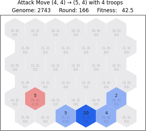
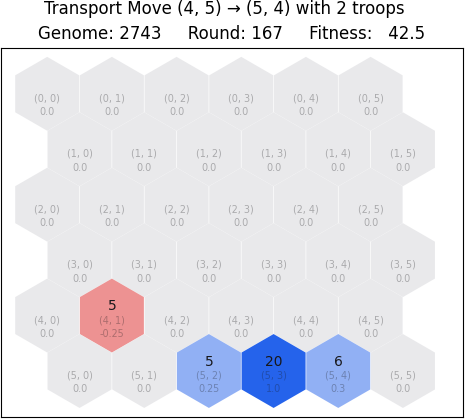
The following example illustrates a case where the blue player decides to transfer troops from origin tile (4, 5) to destination tile (5, 4). Both tiles are neighboring and on the same territory, therefore the transport can be made. After the move is applied, the tile (5, 4) has more troops than before, and the tile (4, 5) is now part of nature.
3. State visualization
For this project, all images of game states are generated using a custom tool. The game_map.py file contains theGameMap class which is used to visualize game states in a two-dimensional space. This class is closely coupled with the Game class along with parameters provided from the NEAT algorithm. In order to generate the required graphics, we utilize matplotlib, a widely used plotting library in Python. Let us begin with an example game state:
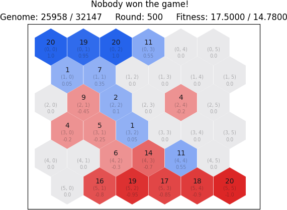
In Figure 3.1 we observe an example game state and how it is represented using the GameMap class. There are three main components: title, subtitle and the map. The title is the first element of the visualization, and it contains vital information about what is depicted on the map. For our case, we see that the title reads "Nobody won the game!", thus we know that we are looking at the end state of a game. In other occasions, we may see "Game Overview" which is the initial state, or descriptions of individual moves applied by the two players. Examples of player moves applied are described as: "Production Move (x, y)", "Attack Move (x1, y1) → (x2, y2) with z troops" and "Transport Move (x1, y1) → (x2, y2) with z troops" where x, x1, x2, y, y1, y2 are tile coordinates and z is the amount of selected troops. The subtitle contains supplementary information that help understand further the current state of the game. We have three items: the genome ids, rounds and fitness. The genome ids are directly taken from the NEAT library and inform us about which genomes are playing the game. The fitness metric is for blue and red and is the overall fitness up to that round. The create_title() andcreate_subtitle() methods are responsible for generating the title and subtitle text respectively. Finally, we have the map which is the final and most complex component.
In order to generate a two-dimensional map of the game state, we call the render() method. This method makes the initial calls to matplotlib in order to create a new plot with the rendering. Once the setup is done, we make individual calls to the render_tile() method for each tile to be displayed on the map. All tiles are represented using the GameMapTile class imported from the game_map_tile.py file. By looking at the attributes of this class, we have four notable tile components: the tile background color, the number of troops, the tile coordinates and the encoding value. These components are used to visualize each tile according to the current game state. TheGameMap class holds a game_map_tiles dictionary that maps tile coordinates to GameMapTile instances. When therender_tile() method is called, the individual tile components are rendered only when changes are detected. Therefore, when the method is first called, the tile is rendered as a whole, but afterwards, only the required components are updated according to game state. This is achieved by storing GameMapTile instances in the dictionary and checking their attributes for updates later in the execution.
When the render() method is called, the game map is displayed in a separate pop-up window that blocks main thread execution. This is a limitation with matplotlib because the plot must run on the main thread. In order to make things simple and convenient, the save() method is used instead to store the map renderings as .png files. This is utilized in the run_inspect.py file, where individual games played by genomes can be re-run and rendered in the games/ folder. The rendered images depict round per round progress of a game and are saved as "round-x-player-y.png" where x is the round number and y is the player id. Conveniently, when each round is saved as an image, we can go both back and forth between game states and inspect the gameplay progress.
4. NEAT parameters
The following options are used throughout this project on all game presets.
| Parameter | Value |
|---|---|
fitness_criterion | max |
| The end goal is to maximize the fitness payoff during the evolutionary process. | |
fitness_threshold | 100 |
| Halt the algorithm after fitness has reached 100%. | |
no_fitness_termination | False |
| The algorithm should not ignore the first two parameters. | |
pop_size | 100 |
| The population is initialized with 100 genomes. | |
reset_on_extinction | True |
| Reset the algorithm in cases where all species become extinct at the same time. | |
species_fitness_func | mean |
| The method of calculating the fitness of a certain species. | |
max_stagnation | 15 |
| The number of generations required for a species to become extinct when there is no improvement on fitness. | |
species_elitism | 0 |
| The number of species to protect from extinction. | |
elitism | 1 |
| The number of most-fit genomes to preserve intact from generation to generation. | |
survival_threshold | 0.2 |
| The fraction of species that are allowed to reproduce on each generation. | |
min_species_size | 2 |
| The minimum number of genomes required to declare a new species. | |
activation_default | sigmoid |
| The default activation function for each node. | |
activation_mutate_rate | 0.0 |
| The probability that a mutation occurs on the activation function of a node. | |
activation_options | sigmoid |
| The list of available activation functions to choose from when a mutation occurs. | |
aggregation_default | sum |
| The default aggregation function for each node. | |
aggregation_mutate_rate | 0.0 |
| The probability that a mutation occurs on the aggregation function of a node. | |
aggregation_options | sum |
| The list of available aggregation functions to choose from when a mutation occurs. | |
compatibility_disjoint_coefficient | 1.0 |
| The coefficient for disjoint and excess genes for the genomic distance formula. | |
compatibility_weight_coefficient | 1.0 |
| The coefficient for weights and bias differences for the genomic distance formula. | |
enabled_default | True |
| New connections should be enabled by default. | |
enabled_mutate_rate | 0.1 |
| The mutation probability for enabling or disabling an existing connection. | |
feed_forward | True |
| Neural networks are feedforward, they do not have recurrent connections. | |
initial_connection | full |
| Initially, all input nodes are connected with all output nodes. | |
node_add_prob | 0.3 |
| The probability of a new node being added to the network. | |
node_delete_prob | 0.3 |
| The probability of an existing node being removed from the network. | |
conn_add_prob | 0.3 |
| The probability of an existing connection being added on the network. | |
con_delete_prob | 0.3 |
| The probability of an existing connection being removed from the network. | |
num_inputs | 36 |
| The number of input nodes on all networks. | |
num_hidden | 0 |
| The initial number of hidden nodes on all networks. | |
num_outputs | 4 |
| The number of output nodes on all networks. | |
bias_init_mean | 0.0 |
| The mean of the gaussian distribution from which initial bias values are selected. | |
bias_init_stdev | 1.0 |
| The standard deviation of the gaussian distribution from which initial bias values are selected. | |
bias_init_type | gaussian |
| Initial bias values are selected from a gaussian distribution. | |
bias_replace_rate | 0.1 |
| The probability of a bias value being replaced with a new one. | |
bias_mutate_rate | 0.9 |
| The probability of a bias value being modified by adding a random value. | |
bias_mutate_power | 0.5 |
| The standard deviation of a zero-centered gaussian distribution from which bias mutation values are selected. | |
bias_max_value | 30.0 |
| Bias values have this upper limit. | |
bias_min_value | -30.0 |
| Bias values have this lower limit. | |
weight_init_mean | 0.0 |
| The mean of the gaussian distribution from which initial weight values are selected. | |
weight_init_stdev | 1.0 |
| The standard deviation of the gaussian distribution from which initial weight values are selected. | |
weight_init_type | gaussian |
| Initial weight values are selected from a gaussian distribution. | |
weight_replace_rate | 0.1 |
| The probability of a weight value being replaced with a new one. | |
weight_mutate_rate | 0.9 |
| The probability of a weight value being modified by adding a random value. | |
weight_mutate_power | 0.5 |
| The standard deviation of a zero-centered gaussian distribution from which weight mutation values are selected. | |
weight_max_value | 30.0 |
| Weight values have this upper limit. | |
weight_min_value | -30.0 |
| Weight values have this lower limit. | |
response_init_mean | 1.0 |
| The mean of the gaussian distribution from which initial response values are selected. | |
response_init_stdev | 0.0 |
| The standard deviation of the gaussian distribution from which initial response values are selected. | |
response_init_type | gaussian |
| Initial response values are selected from a gaussian distribution. | |
response_replace_rate | 0.0 |
| The probability of a response value being replaced with a new one. | |
response_mutate_rate | 0.0 |
| The probability of a response value being modified by adding a random value. | |
response_mutate_power | 0.0 |
| The standard deviation of a zero-centered gaussian distribution from which response mutation values are selected. | |
response_max_value | 1.0 |
| Response values have this upper limit. | |
response_min_value | 1.0 |
| Response values have this lower limit. | |
compatibility_threshold | 3.0 |
| Genomes with genomic distance less than this value are in the same species. | |
5. Neural network input and output
For the purposes of this project, all neural networks are initialized with 36 input neurons, no hidden layers and 4 output neurons. Inputs are initially fully connected with all outputs. The state_parser.py file contains the StateParser class which is responsible for encoding game state input for neural networks and decoding player moves from neural networks. The encode_state() method captures the current game state and returns a vector of values in [0, 1]. This vector holds encoded values for each tile of the map. These values are calculated by taking the number of troops present on the tile and dividing that value with the maximum number of troops on each tile. The value is positive if the tile is owned by the blue player and negative if owned by the red player. Let us demonstrate an example:
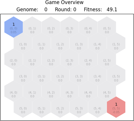
As observed in Figure 5.1 each tile holds an encoded value in the game state representation. For tile (0, 0) we see that the value is 0.05 and for tile (5, 5) the value is -0.05. We know that the maximum number of troops allowed on each tile is 20, therefore if we do the division, the encoded value is correct. The red tile holds a negative value, since it is owned by the red player. As the rest of the map belongs to nature, we observe that the encoded values are zero, since there are no troops present on grey tiles. Considering the size of the map, the neural network receives a vector that holds 36 values:
[0.05 0.0 0.0 0.0 … 0.0 -0.05]
Let us review another example, where blue and red tiles are spread across the map.
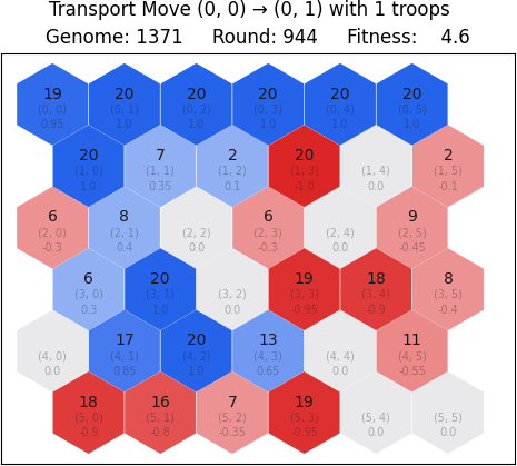
In Figure 5.2 we observe the state of a game after a considerable number of rounds. Both players are spread across the map, therefore it is worth looking at how the game state is depicted in vector form:
[0.95 1.0 1.0 1.0 … -1.0 0.0 -1.0 … 0.0]
This is essentially what the neural networks see. The current game state is depicted in vector form, and then passed on as input every time a new move is requested. Positive and negative representations help to distinct the difference in tile ownership. A zero value always encodes a tile owned by nature, whereas a positive or negative number signifies that the tile is owned.
The decode_state() method is used to decode the output of neural networks. It accepts a one-dimensional vector containing values in [0, 1]. The values originate from the output neurons of neural networks and are translated to valid game moves. The output vector is comprised of four different components: production flag, source tile, target tile and troop count. These components are extracted and parsed in different ways. The production flag is a boolean value that signifies whether the output should be treated as a production move. The source and target tile components represent the tile of origin and destination for cases of attack and transport moves. Finally, the troop count is the number of troops to be selected from the source tile.
In order to extract these components, we use the decode_prod_flag(), decode_tile() and decode_troops() methods. The first method is used to parse the production flag. It performs a single check, whether the output value is smaller or equal to 0.5. We end up with the desired boolean value. The second method is used to parse the source and target tile components. It divides the [0, 1] space to 36 distinct subspaces with lower and upper bounds. We then compare the output with each space to decide which one of the 36 tiles should be selected. Similarly, the third method maps the [0, 1] space to 20 distinct subspaces, which is the maximum number of troops that can be selected.
The next step is to decide which type of move is desired, depending on the individual components that are extracted. There are four types of move enumerations: IdleMove, ProductionMove, AttackMove and TransportMove. Depending on which one will be selected, the appropriate game move is applied. First, if the production flag is set to True and a potential production move is valid (according to the game rules), then the ProductionMove is selected. Next, if the previous choice is not plausible, we check for a potential attack or transport move. If one of the two can be made, the AttackMove or TransportMove is selected, respectively. Finally, if none of the previous options are valid, we select the IdleMove enumeration, and the move is considered invalid. The validity checks are performed by calling the is_production_move_valid(), is_attack_move_valid() andis_transport_move_valid() methods from the Game class.
If the move enumeration is decided, we apply the respective game move. However, for invalid moves, we add an extra step. Because invalid moves have no effect on the game, there needs to be a way to progress without making the player stay idle. For example, the output vector might suggest that the player should attack tile (3, 3), but the tile might be out of reach. The parsing is valid, but according to game rules the move is invalid. Consequently, in order to avoid such cases, we guide the player into selecting the closest valid move.
The guide_move() method is responsible for turning an invalid move into a valid one. First, the get_next_moves()method is called in order to generate a list of all possible valid moves depending on the current state of the game. In order to create that list we go through a process of calculating next game states based on applicable moves. Once we have that list, we then compare each move with the invalid one, by calculating the Euclidean distance with three components: source tile, target tile and troop count. The move with the smaller distance is selected. Finally, the decode_state() method returns the valid guided move, instead of the original.
[0.0 0.04411154570991824 0.9999687598147949 0.9999999999980089]
We begin by parsing the production flag component by looking at the first element of the output vector. Since the value is less than 0.5, the production flag is True. Next, we look at the second element, to extract the source tile component. As mentioned earlier, there are 36 options. Therefore, after mapping the number to the correct subspace we select the (0, 1) source tile. As for the other target tile and troop count components, they will be ignored since production moves require only the source tile component. Now that the output vector is parsed, we call the is_production_move_valid() method to check whether this move can be made. Assuming the method returns True, we end up with the following dictionary object describing the move:
player_move = {
    "move_type": Game.ProductionMove,
    "source_tile": (0, 1),
    "target_tile": (0, 1),
    "troops": 1,
    "guided": False
}
Let us review a second example. For this case, we use an output vector that results in an invalid game move.
[0.7583775969117601 0.09880653506612425 0.9956816595680481 0.9999999999999927]
Once parsed, we have the following representation:
player_move = {
    "move_type": Game.IdleMove,
    "source_tile": (0, 3),
    "target_tile": (5, 4),
    "troops": 20,
    "guided": False
}
If we look at the game state, we notice that the player move cannot be applied.
Looking at Figure 5.3 and Figure 5.4 the tile at (0, 3) is owned by the blue player, however tile (5, 4) is not neighboring with any of the player’s tiles. Therefore, the move is not valid. After applying the guide_move()method, we end up with the closest possible valid move:
player_move = {
    "move_type": Game.AttackMove,
    "source_tile": (0, 2),
    "target_tile": (1, 2),
    "troops": 19,
    "guided": True
}
By looking at the two examples, it is evident that the neural network output always translates to a valid game move. Having that in mind, the whole training process is simplified, because we are not forced to end the game after coming to a dead end. Even if the neural network is unsure about a certain situation, we always find the closest possible move, therefore any output given will alter the state of the game in some way.
6. Training cases
On this project, we study applications of the NEAT algorithm by allowing networks to train on five different game presets. The first case puts the blue player into the test, by initializing the game with an empty map for blue with the absence of the red player. The second and third cases introduce a challenge for blue, by placing red tiles on the map, without allowing the red player to take turns. In fourth case, we allow both players to play, but the red player selects moves based on a deterministic move selection algorithm. Finally, we coevolve both blue and red players, by making neural networks play against each other.
As briefly mentioned in Game overview, in order to create training cases that share common rules, we use game presets. The game_presets.py file includes four classes based on the Game class: BlueExpandAlone,BlueBeatRedEasy, BlueBeatRedHard and BlueAgainstRed. These subclasses encode the cases mentioned respectively, by implementing custom methods for map initialization, game settings, fitness functions and win conditions. The fifth case is treated different, as it is a separate project on its own (based on the original) due to the vast differences in implementation.
The run_evolve.py is a runnable Python file that is used to start or resume the execution of the NEAT algorithm. By providing an optional preset flag (-p, --preset [1, 2, 3, 4]), we choose which type of preset we want to evolve. As mentioned in NEAT parameters, we initialize the learning algorithm with 100 neural networks for an infinite number of generations to run. After each generation, we save the current progress in a checkpoint file, inside folders starting with the checkpoint prefix. Furthermore, we record information about game runs in JSON format. These files are included in folders starting with the game-result prefix. Lastly, the entire gameplay process for each fitness evaluation is done using the multithreading library in Python. That way we can speed up the process by processing multiple games in different CPU cores on the host computer.
Each training case has different win criteria; however, all matches are subject to termination if the game is deemed to be stale. When one state is repeated more than three times, then the game is stopped. This mechanism is present, in order to prevent neural networks from applying the same move repeatedly without any purpose.
6.1. Blue player on an empty map
We start with a simple case, where the blue player is placed on the upper left corner of an empty map. The red player is absent, and the end goal for blue is to take over the entire map as soon as possible. There is no competition for blue, therefore it is only a matter of learning how to play game. The initial state for all neural networks in the population is depicted in Figure 6.1.
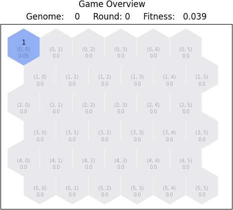
The round limit is set to 5,000 and the blue player wins if the entirety of the map is conquered. We define a fitness function for this case with the following criteria:
- For all cases, claim up to 50% of the maximum fitness depending on the number of tiles you have conquered from 36 total.
- If blue player won, claim up to 50% of the maximum fitness depending on the number of rounds the game lasted before conquering the entirety of the map.
The two fitness component values are squared and then summed, so we can build up a higher fitness payoff as the blue player converges towards end goal. We end up with a percentage and the maximum ideal fitness of 100%.
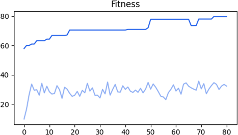
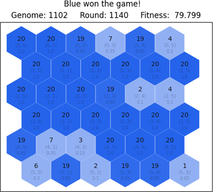
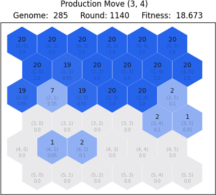
After running for 80 generations, the most fit network has a fitness payoff of 79.7%, conquering the entirety of the map after playing for 1,140 rounds. The topology of the neural network contains 36 input neurons, 7 hidden neurons, 4 output neurons and 150 connections. The second and third best neural network complete the task after 1,754 and 1,843 rounds, respectively. In the following graph, we observe the fitness progression through generations. The upper blue plot depicts the fitness of the most fit network, and the lower light blue plot depicts the average fitness of the entire population.
The most-fit network developed a gameplay style that involved 568 production moves, 43 attack moves and 529 transport moves. From the 1,140 moves in total, 636 moves were guided, meaning that the program used the correction gate for most of the moves in order to end up on valid ones.
In order to observe the learning curve of the population, let us look at the differences between the first and second best network. We render the game state of round 1140 – which is the final game state for the most fit network – to note the differences in map ownership. Looking at Figure 6.3 and Figure 6.4 it is evident that in the first case, the game has already ended since blue player conquered all 36 tiles, whereas in the second case, the blue player has only conquered 22 tiles. This difference in gameplay makes the first player considerably better than the second one, as both the number of tiles and rounds are fitness components. The major difference in fitness (79.7 and 18.6) is caused because of the rounds component, as it is rewarded only when blue player wins.
6.2. Blue player against easy red
The second case introduces a different challenge for blue, by adding the red opponent on the map. The red player remains static, without reacting to any moves applied by the blue player. The end goal for blue is to eliminate all red tiles as soon as possible. In Figure 6.5 we look at the initial map setup where the red player owns 6 tiles with 40 troops.
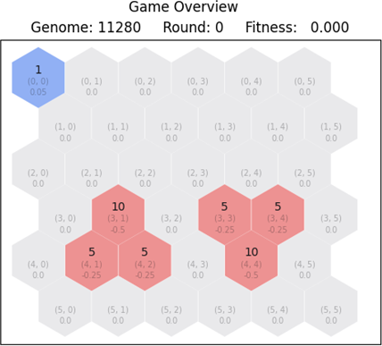
The round limit is set to 500 and the blue player wins only when all 6 tiles owned by red are eliminated. We define a fitness function for this case with the following criteria:
- For all cases, claim up to 30% of the maximum fitness depending on the number of tiles blue has conquered from red.
- For all cases, claim up to 20% of the maximum fitness depending on the number of troops blue has killed from red.
- If blue player won, claim 20% for the victory.
- If blue player won, claim up to 30% of the maximum fitness depending on the number of rounds the game lasted before eliminating red.
The final fitness is the sum of the four individual components. We end up with a percentage and the maximum ideal fitness of 100%.
After running for 261 generations, the most fit network has a fitness payoff of 93.8%, defeating red after playing for 102 rounds. The topology of the neural network contains 36 input neurons, 6 hidden neurons, 4 output neurons and 114 connections. The second and third best neural network complete the task after 108 and 136 rounds, respectively. In the following graph, we observe the fitness progression through generations. The upper blue plot depicts the fitness of the most fit network, and the lower light blue plot depicts the average fitness of the entire population.
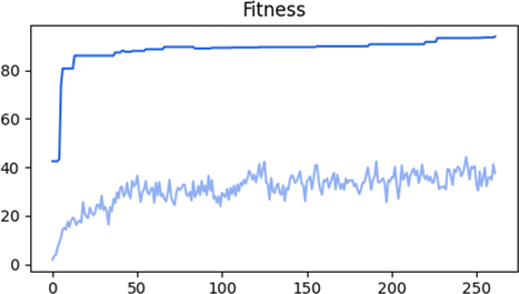
Since the number of moves is relative to the number of rounds, it is evident that the blue player is more than capable of defeating the red player. The most-fit network managed to complete the task, with just 66 production moves, 28 attack moves and 8 transport moves.
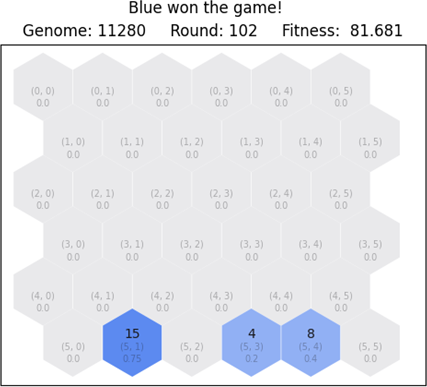
Like the comparisons from the first case, let us look at the first, second and third best network. We render the game state for the final round 102, in order to look at the differences in gameplay. Looking at Figure 6.7 , Figure 6.8 and Figure 6.9 we notice that the first network has successfully defeated red. However, the second and third network have yet to complete the task after the round of interest. Furthermore, on the second case there is 1 red tile left. Likewise, on the third case, there are 4 red tiles left.
6.3. Blue player against hard red
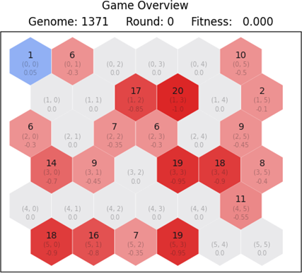
The third case introduces a challenge harder than the one described in the second case. The blue player is given the task of eliminating red; however, the number of red tiles is significantly larger. The red player remains static throughout the game, without reacting to any of the moves applied by blue. In Figure 6.10 we look at the initial setup where the red player opponent starts off with 19 tiles and 222 troops.
The round limit is set to 5,000 and the blue player wins only when all 22 tiles owned by red are eliminated. The upper round limit is greater compared to the second case, due to the extra difficulty of this task. We define a fitness function with the following criteria:
- For all cases, claim up to 30% of the maximum fitness depending on the number of tiles blue has conquered from red.
- For all cases, claim up to 20% of the maximum fitness depending on the number of troops blue has killed from red.
- If blue player won, claim 20% for the victory.
- If blue player won, claim up to 30% of the maximum fitness depending on the number of rounds the game lasted before eliminating red.
The final fitness is the sum of the four individual components. We end up with a percentage and the maximum ideal fitness of 100%.
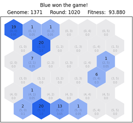
After running for 128 generations, the most fit network has a fitness payoff of 93.8%, defeating red after playing for 1,020 rounds. The topology of the neural network contains 36 input neurons, 2 hidden neurons, 4 output neurons and 116 connections. The second and third best neural network complete the task after 1,065 and 1,101 rounds, respectively. In the following graph, we observe the fitness progression through generations. The upper blue plot depicts the fitness of the most fit network, and the lower light blue plot depicts the average fitness of the entire population.
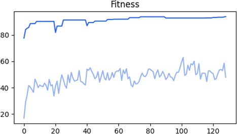
Despite the challenge, the most-fit network managed to beat the red player after 313 production moves, 109 attack moves and 598 transport moves. The blue player focused on eliminating red after building up the necessary forces. Since the red player is not reacting to any moves, blue has all the time to build up without the need of defending attacks or considering changes in red forces.
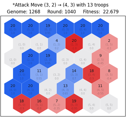
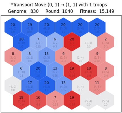
Let us look at the first, second and third best network, like the comparisons from previous cases. We render the game state for the final round 1,020 in order to look at the differences in gameplay. Looking at Figure 6.12, Figure 6.13 and Figure 6.14 we notice that the first network has successfully defeated red. However, the second and third network have yet to complete the task after the round of interest. Furthermore, on the second case there are 10 red tiles left. Likewise, on the third case, there are 13 red tiles left.
6.4. Blue against deterministic red
The fourth case differs from the first three scenarios, as the red player no longer remains static throughout the game. Based on the game state of each round, red selects an appropriate move based on a deterministic algorithm. The blue player is controlled with a neural network and is tasked to eliminate the red player from the map. For this case, we utilize the Generator class from the numpy package in order to create a deterministic random number generator. That way, for all training cases, the red player is predictable as it will always react the same when a certain game state is evaluated. Let us look at the initial state depicted in Figure 6.15.
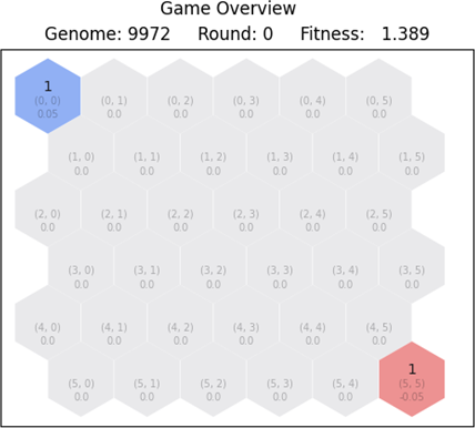
The round limit is set to 500. During a match, the blue player always takes turns from neural network activations, whereas the red player selects moves based on certain criteria. The available pool of next moves is generated for red, by looking at the current game state for each round. We define the following move selection criteria for red:
- If the number of blue tiles is greater than the number of red tiles and red player can make an attack move, select a random attack move.
- Otherwise, if the number of red troops is less than 20 or less than the number of blue troops and red player can make a production move, select a random production move.
- Finally, if the criteria above are not satisfied, select a random move.
Now that we have laid the ground rules for red, let us look at the fitness function for blue:
- For all cases, claim up to 50% of the maximum fitness depending on the number of tiles blue has conquered overall.
- If blue player won, claim up to 50% of the maximum fitness depending on the number of rounds the game lasted before eliminating red.
The final fitness is the sum of the two individual components. We end up with a percentage and the maximum ideal fitness of 100%.
After running for 162 generations, the most fit network has a fitness payoff of 65.1%, defeating red after playing for 99 rounds. The topology of the neural network contains 36 input neurons, 2 hidden neurons, 4 output neurons and 137 connections. The second and third best neural network complete the task after 61 and 84 rounds, respectively. In the following graph, we observe the fitness progression through generations. The upper blue plot depicts the fitness of the most fit network, and the lower light blue plot depicts the average fitness of the entire population.
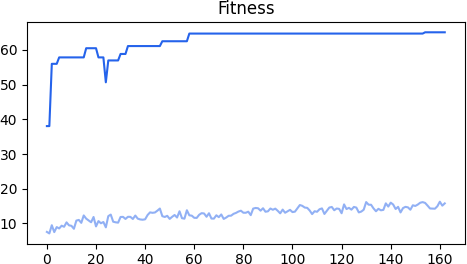
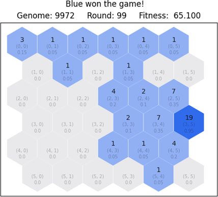
It turns out that the blue player was more than able to defeat red. Considering that blue was expected to win the game and conquer as many tiles as possible, the result is satisfactory. After 62 production moves, 31 attack moves and 6 transport moves, 73 of which were guided, blue has defeated red and conquered a total of 18 tiles. The second and third best networks won with 15 and 16 tiles, respectively. In Figure 6.17 we look at the end state for the most fit network.
6.5. Coevolution of blue and red player
For the fifth and final training case, we introduce two neural networks for blue and red, respectively. In all previous cases, blue was the only player controlled with a neural network. Now, we task two neural networks to play against each other, until one eliminates the other. We go through a process of coevolution, where both populations repeatedly play games against each other, striving for a large fitness payoff. Let us study the implementation details, first by looking at the initial state depicted in Figure 6.18.
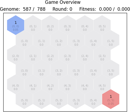
The blue player – just like the previous training cases - starts on the upper left corner and the red player on the lower right corner. In order to evaluate individual fitness, we must first go through a process of matching every network on the blue population with a network on the red population. Since the two populations can grow or shrink in size due to the reproduction of species from generation to generation, we have three distinct cases. If the two populations are equal, then blue and red networks can be matched one to one. If the blue population is larger, then the blue networks are matched with the red ones, and the extra networks are matched with a random network from red. Similarly, if the red population is larger, then red networks are matched with blue ones, and the extra networks are randomly matched with blue networks.
As mentioned in the introductory of this chapter, we process games in a multithreaded manner. This gives us great flexibility, as we can run two populations and evaluate individual fitness in parallel as games are concluded. We initialize two populations for blue and red, and for each generation, we have a one-to-one match for all networks. Once all games in a generation have ended, fitness is assigned for the blue and red networks as if they were playing solo. The networks are not aware of the presence of other networks. The only difference is visible in game state, as it can now be altered in a non-deterministic manner. Let us look at the fitness function for this training case.
Instead of calculating the overall fitness at the end of each game, we now evaluate fitness per move. This is done so we can search for desired behavior by inspecting every detail of the player’s strategy. At the end of each game, we calculate the final fitness by taking the average of the per-move fitness for both blue and red. This type of fitness is based on four components: tiles gained, troops gained, enemy tiles conquered, enemy troops killed. These four components express 100 different outcomes with the application of any type of move. For example, selecting a production move would encode vector (0, 1, 0, 0) meaning that the second component for troops gained is set to 1. Or, if the player selects an attack move, the resulting vector (0, -5, 0, -5) suggests that the player launched an attack that led to 5 troop kills for both players.
For each vector we assign a fitness payoff depending on how beneficial the outcome of the move turned out. We start with the lowest fitness payoff for vector (-1, 0, 0, 0) and end with the highest fitness payoff for vector (1, -19, -1, -19). The worst possible move for a player is to lose a tile after applying a move, whereas the best possible move is to conquer an enemy tile after killing a maximum of 19 of their troops. The main difference compared to other training cases, is that instead of calculating a predefined percentage of an end goal (ex. conquering red’s static tiles), we now evaluate the performance of individual moves. In order to prevent games from progressing infinitely, we set an upper round limit of 5,000 rounds. Since both players are given the same task, it is apparent that if one player evolves to make better moves, eventually the opponent will also improve. Both players are set to maximize fitness, therefore the two players drive each other into making better moves.
After running for 25 generations, the blue most fit network has a fitness payoff of 231 and the red most fit network has a fitness payoff of 191. Both blue and red networks played for 5,000 rounds. The topology of the blue network contains 36 input neurons, 3 hidden neurons, 4 output neurons and 146 connections. Similarly, the red network has 36 input neurons, 3 hidden neurons, 4 output neurons and 136 connections. In the following graph, we observe the fitness progression through generations. The upper blue and red plots depict the fitness of the most fit blue and red networks. The lower light blue and red plots depict the average fitness of the blue and red population.
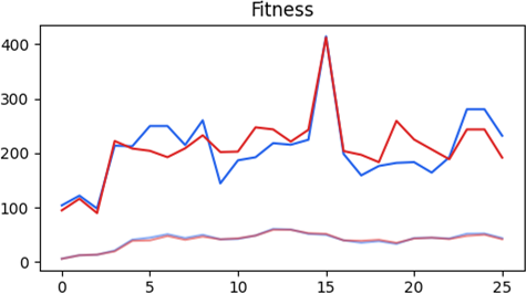
By looking at Figure 6.19 we notice an interesting spike on the 15th generation. The most fit individuals peaked at a fitness of 414 for blue and 412 for red. Why is it that the fitness dropped right after this generation? There may be plenty of reasons as to why this happened, the most probable case being a mutation on either blue or red, that changed the course of the next games. If we compare the moves of most-fit individuals from the 15th and 25th generation, we notice that both players in the 15th generation launched a considerable number of attacks compared with the 25th generation. Furthermore, the transport moves were chosen way less compared to the other two moves. For the 15th generation blue had 2,881 production moves, 1,630 attack moves, and 481 transport moves. Red had 2,867 production moves, 1,322 attack moves and 810 transport moves. For the 25th generation blue had 1,106 production moves, 1,053 attack moves and 2,841 transport moves. Finally, red had 1,294 production moves, 260 attack moves and 3,445 transport moves.
By looking at the gameplay between the most-fit blue and red genomes from the 15th generation, we notice something interesting. Let us investigate further by rendering two rounds of interest: 2,500 and 5,000 in Figure 6.20 and Figure 6.21, respectively.
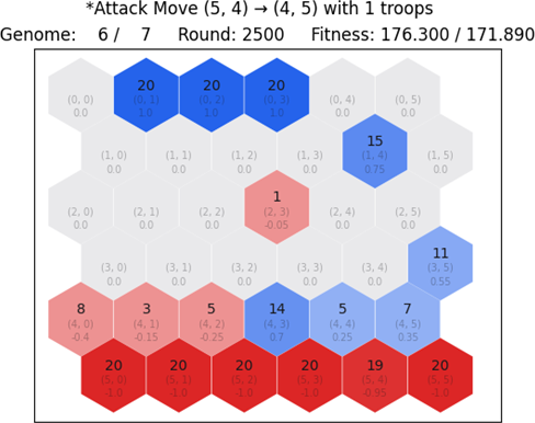
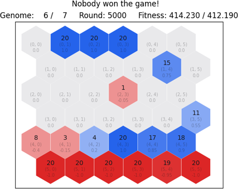
We notice that the game state from round 2,500 up to round 5,000 is slightly different yet almost the same. However, the only real metric that is changing is the fitness payoff. By looking at the sequence of moves applied from both players, there seems to be a pattern that suggests cooperation. We expected that the blue player would be the rival of red, but it appears that instead of fighting over dominance, the neural networks developed a different approach. This is the case for the 15th generation, as the two players instead of fighting, they have discovered a strategy that exploits fitness and developed a pattern of cooperation. Both players receive a fitness payoff by either gaining or losing tiles and troops. In the long run, we realize with surprise that both players benefit from each other instead of one trying to harm one other.
These patterns of cooperation have been observed, whilst trying different types of fitness functions. For example, if we were to reward transport moves, it is possible that a neural network would rise in fitness by exploiting this payoff. There is no rule in the game that prevents one from transporting troops back and forth between tiles, therefore, if the transport move is rewarding, it can and eventually will be exploited. The same can be concluded for attack moves, but with a twist. One may not be able to attack themselves, however, no one is stopping players from attacking one another. Since there is no pre-programmed sense of rivalry nor competition, this feature can also be exploited to an extent. Both the blue and red player can mutually agree on a strategy of attacking one another; and then rebuilding, only for the purpose of stealing the fitness payoff.
Originally, when designing the fitness function for this scenario, the intent was that the blue player would start attacking red and vice versa. However, this is how it could work, and not how it works. The objective of the NEAT algorithm for our project is to evolve neural networks capable of maximizing the given fitness function. If that function allows for cooperation between the two players, then it is certain that at some point this behavior will be tested in action. Even though games can be terminated when deemed to be stale, it appears that the neural networks have not only cooperated but also found a way of keeping the game alive. The result may have not been desired, but since the fitness of both networks significantly increased, technically the algorithm did work.
7. Conclusions
On this project, we studied applications of the NEAT algorithm by creating a simple two-dimensional board game in Python. We laid some basic rules and moves for the two players and we setup five different training cases. We used popular third-party libraries from the Python community that helped with the rapid development of the game. After running NEAT for a considerable amount of time, we have made remarks on the performance of our experiment. The four training cases placed blue against a deterministic opponent and was able to approximate the fitness function in a satisfactory level. The fifth training case tested both blue and red in a coevolutionary environment. Both players were tasked with defeating one another, however we observed the development of a pattern of cooperation. All cases were of varying difficulty, each one with a unique twist. It appears that the neural networks were most efficient in cases where the opponent remained static throughout the game.
This simple board game required a fair amount of computational power, due to the vast number of games that were played concurrently. This factor is limiting, as the training environment can always make use of better hardware. We used the multithreading package, which helped significantly with the training process. However, as we know, Python is an interpreted language hence the processing power is limited. Rewriting the entire project in a compiled language such as C++ could offer major performance improvements. Furthermore, different types of fitness functions could be tested for all training cases. Perhaps a difference in fitness may render more effective results than the ones presented. Lastly, alternative vector representations could be tested for encoding game state, as well as decoding moves from neural network outputs.
8. References
[1] K. O. Stanley and R. Miikulainen, "Evolving Neural Networks through Augmenting Topologies," The MIT Press Journals, vol. 10, no. 2, pp. 99-127, June 2002.
[2] X. Yao, "Evolving Artificial Neural Networks," Proceedings of the IEEE, vol. 87, no. 9, pp. 1423-1447, September 1999.
[3] D. Chen, C. L. Giles, G. Z. Sun, H. H. Chen, Y. C. Lee and M. W. Goudreau, "Constructive Learning of Recurrent Neural Networks," IEEE International Conference on Neural Networks, pp. 1196-1201, 1993.
[4] J. D. Schaffer, D. Whitley and L. J. Eshelman, "Combinations of Genetic Algorithms and Neural Networks: A Survey of the State of the Art," COGANN-92: International Workshop on Combinations of Genetic Algorithms and Neural Networks, pp. 1-37, 6 June 1992.
[5] A. McIntryre, M. Kallada, C. G. Miguel and C. F. d. Silva, neat-python.